This article presents an analytic method of dividing a round horn into several segments, so that the cross section of the horn is no longer circular everywhere, but transforms into a sharp-edged polygon at some point along its axis, and then back to circle again. This may come handy e.g. when assembling a horn from several pieces, but here we don't deal further with the reasons but solely with the applied method itself.
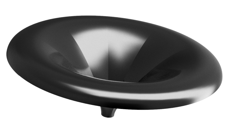
Even though the described method is quite general and applicable to many other devices, we will show its use on a R-OSSE, free-standing waveguide (see Fig.1).
In the following we will use a cylindrical coordinate system as \((r,\theta,z)\), with its axis being the axis of the horn, \(z=0\) being the plane of the throat.
For the purpose of this article, we will use a R-OSSE waveguide [1] defined as follows:
\(R = 200 mm, r_0 = 12.7 mm, a = 35°, a_0 = 5°, k = 1.5\)
For being axisymmetric, such horn can be described simply as \([r(t), \theta, z(t)]\), i.e. independently of \(\theta\)
(remember that a R-OSSE is a parametric curve for \(0 \le t \le 1\),
it can't be described merely as \([r(z), \theta, z]\)).
The whole procedure of segmentizing is to take a single sector of the horn for \(\theta\) in a chosen range, and find a transformation \(r(t) \rightarrow r'(t, \theta) \) so that the resulting shape has the desired properties. Without loss of generality, we will use a range \(\langle 0, \theta_S \rangle\) in the rest of the text, with angular span \(\theta_S = 60°\) as an example. Hence, the new segment will be described as follows:
\([r'(t,\theta), \theta, z(t)]\)The task now is just to find the right \(r'(t,\theta)\). For that, we first need to be exact of what we want: At a certain \(z\) (or \(t\) in our case - let's denote it \(t_m\)), instead of a circular arc in the cross section (which is given by the axisymmetric nature of the original shape), we want a straight line (see Fig.2).
It is straightforward to derive the radius term for the line segment in the cross section shown above:
Where \(r_S\) is the chosen radius coordinate of the line segment at the edge of the horn segment.
In this example \(r_S\) = \(r(t_m)\) (both roughly 64 mm), but in general these values are independent.
We will come back to this later.
What is still missing is the dependence on \(t\), as we currently have the correct \(r'\) only for a single selected cross section, i.e. for \(t\) fixed. The idea now is to keep the throat and the mouth intact, and only smoothly vary the applied amount of transforamtion in between, so that at the selected cross section we have the exact solution shown above. To achieve this, we simply add weighting to \(r'(\theta)\) that is dependent on \(t\). One such convenient weighting function with the desired properties is the following one:
\(m(t) = sin \left( \pi \left( {\cfrac{t - t_0}{t_1 - t_0}} \right) ^{\zeta} \right)^\kappa \) for \(t_0 \lt t \lt t_1\), and \(m(t) = 0\) otherwise, \( \qquad (2) \)where \(\zeta\) is a skew and \(\kappa\) is a sharpness of the weighting function, both being user-defined parameters (see Fig.3). In fact, this is just a modified meander function introduced in [2]. Parameters \(t_0, t_1\) have been added to optionally restrict the transformation to a smaller range of \(t\). The weighting is not symmetric for lower and higher values of \(\zeta\), but it may be easily used reversed for \(\zeta > 1\).
The only thing we have to be careful about is that \(m(t)\) has its maximum amplitude at \(t_m = t_0 + \cfrac{t_1 - t_0}{2^{1/\zeta}} \), so this value of \(t\) also defines the reference cross section.
Now we can finally write the formula for the transformed radius:
\(r'(t,\theta) = r(t) + m(t) (r'(\theta) - r(t_m)) \qquad (3)\)
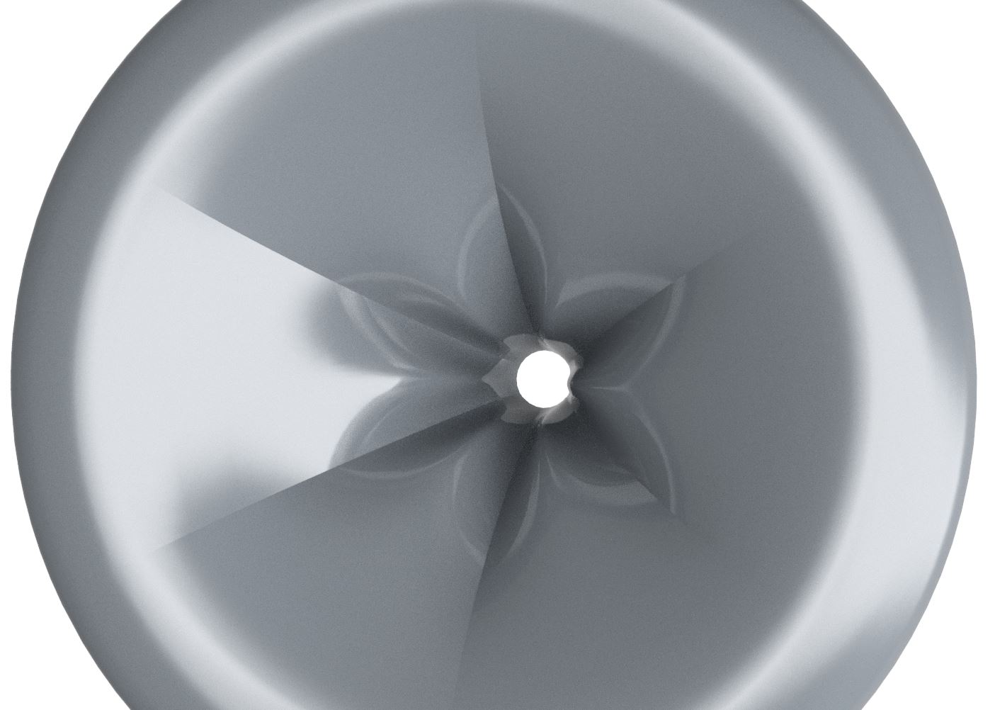
Fig.4A shows a final transformed segment using all the above apparatus.
The original circular arc is still shown but now the surface goes through the blue straight line instead.
The other parameters used were \(t_0=0.8, \kappa=4, \zeta=0.75 \rightarrow t_m \approx 0.32 \).
Fig.4B shows the applied "corrective" term to \(r(t)\).
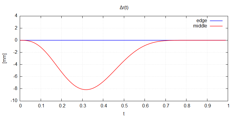
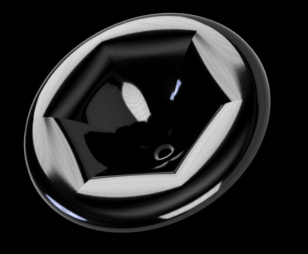
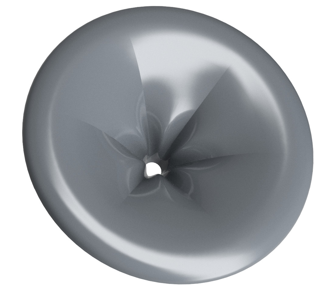
As was mentioned earlier, the parameter \(r_S\) is actually independent of \(r(t_m)\). In the above example, where both were equal, the segment was transformed so that the edges were not changed at all, and the biggest "deformation" was applied in the middle of it. This is advantageous if segments of different angular spans (\(\theta_S\)) are to be assembled together, so that the edges still perfectly match, but it would be easily the other way around if we simply set \(r_S = r(t_m) / cos(\theta_S / 2)\), see Fig.5. Now the middle part stays intact and the transformation is performed towards the edges.

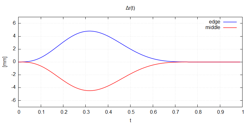
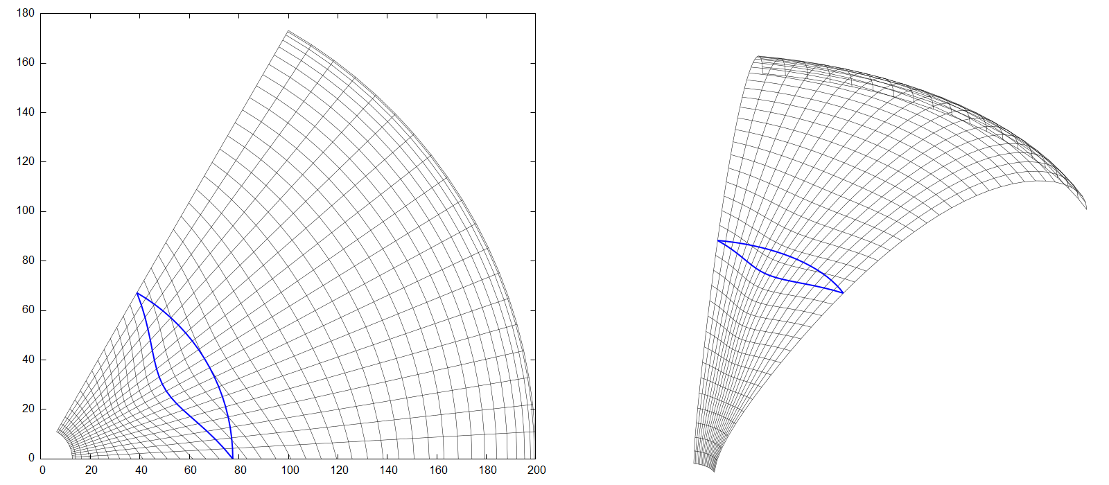
It is also possible to set \(r_S\) to any other value, for example to the geometric average of the above values (Fig.6):
\(r_S = r(t_m) \sqrt{1 / cos \left( \cfrac{\theta_S}{2} \right) }\)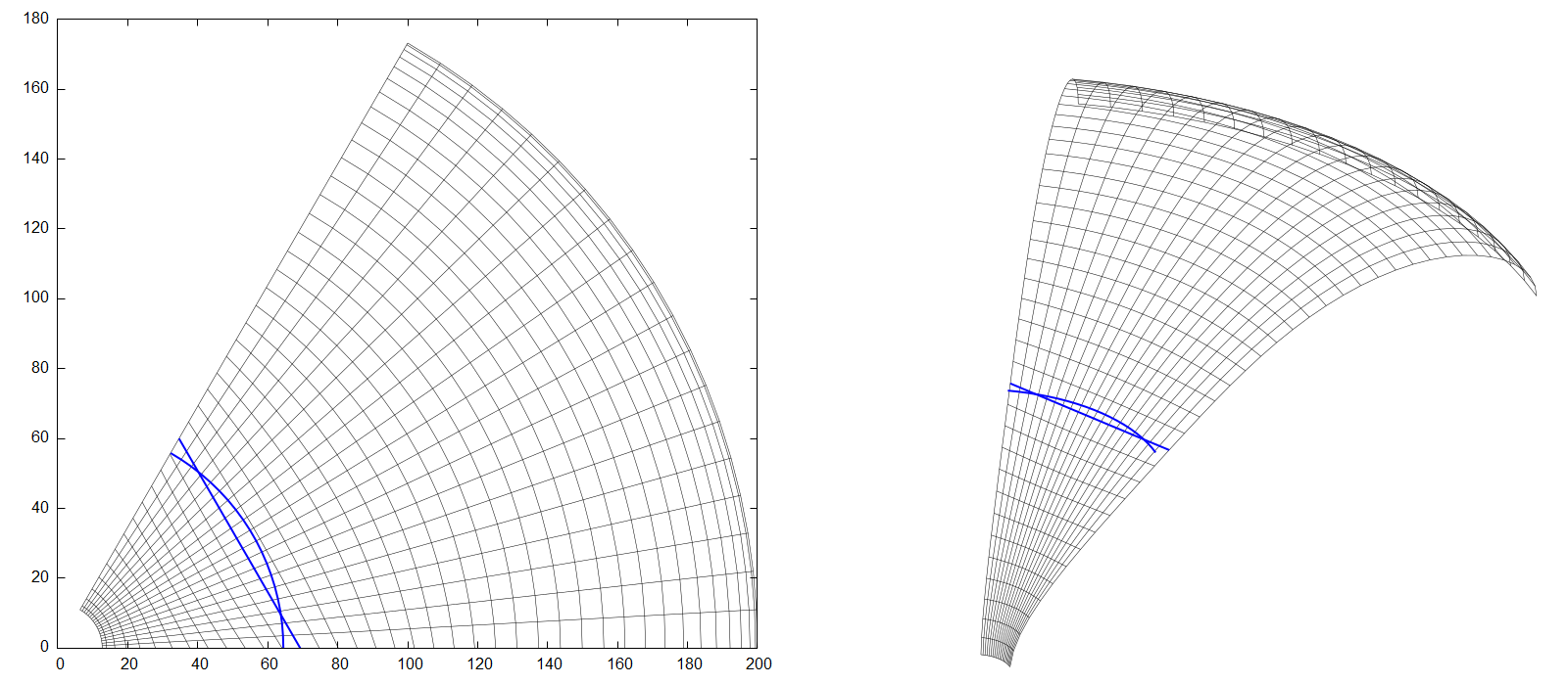
There is of course much more freedom in selecting a function for the \(r'(\theta)\), which is the target radius. For a straight line, we used formula (1). Instead, we can, for instance, use a slightly modified meander function again:
\(r'(\theta) = r_S + \delta \cdot sin \left( \pi \left( {\cfrac{\theta}{\theta_S}} \right) ^{\mu} \right)^\nu \qquad (4) \)The parameter \(\delta\) is the desired amplitude [mm]. Fig.7 shows an example of such target function.
As should be obvious by now, basically any axisymmetric horn can be easily segmentized with the described method, and the individual segments can span arbitrary angles. The method simply takes segment by segment and applies the necessary transformation. In its most basic form it has only two parameters (Fig.3):
\(\zeta = \) skew of the weighting functionWe also presented one of possible generalizations.